Impact of Atmospheric Forcing on Antarctic Continental Shelf Water Masses

Info

• University College London, United Kingdom
• PDF: pettythesis.pdf

Citation

A. A. Petty (2014), Impact of Atmospheric Forcing on Antarctic Continental Shelf Water Masses, Doctoral Thesis, University College London, http://discovery.ucl.ac.uk/1417883/.

Abstract

During my PhD, I developed and analysed climate models of varying complexity. I used both an idealised sea ice-ocean model I developed during my PhD, and a more complex sea ice climate model component (CICE) developed at Los Alamos.

The main aim of the PhD was to understand the cause of regional variability in the properties (e.g. temperature) of the Antarctic shelf seas. See below more for more background on this work.

I was supervised during my PhD by Daniel Feltham (Reading University) and Paul Holland (British Antarctic Survey).

The Antarctic Shelf Seas

Surrounding Antarctica is a region of shallow ocean, where the vast Antarctic ice sheet extended northwards during previous glacial maxima, depressing the sea floor. This shallow shelf sea (although unusually deep compared to continental shelves found elsewhere in the Earth) is a crucial component of the Earth’s climate system. In the western Antarctic we see wide and pronounced shelf seas, which also show a distinct bimodal distribution in the ocean temperature at the seabed (see figure below). It is not clear why this is so.

Circumnavigating Antarctica in a clockwise direction is the largest current in the Earth’s oceans - the Antarctic Circumpolar Current (ACC), which carries relatively warm waters unimpeded through the three great ocean basins (Pacific, Atlantic and Indian).

In the Amundsen and Bellingshausen seas, virtually unmodified Circumpolar Deep Water (CDW) from the ACC floods onto the continental shelf (through various processes). These warm ocean currents are strongly implicated in the recent thinning and acceleration of the Pine Island Glacier, along with several other (less popular!) ice shelves fringing the West Antarctic Ice Sheet.

In the Weddell and Ross seas, large cyclonic gyres mix the ACC with cold surface waters, cooling the water before it floods on to the continental shelf. Cold, near-freezing surface waters then sink to the shelf seabed every winter through sea ice growth (explained in the Sea Ice and Mixed Layer sections below), filling the shelf sea with very cold and saline waters. This cold, High Salinity Shelf Water (HSSW) crosses the shelf break and sinks down to the deep ocean forming Antarctic Bottom Water (AABW), a crucial component of the global thermohaline circulation.

Crucially, we see the surface mixed layer deepen to the shelf seabed in the WR seas, but NOT in the AB seas. Understanding the cause of this bimodal behavior was a main motivation of the PhD

Sea Ice-Ocean Modelling

Idealised Modelling

During the first half of my PhD, I developed an idealised sea ice-mixed layer model (see first figure below). The model comprises three main components: (i) surface energy balances at the ice-atmosphere and ocean-atmosphere interfaces, (ii) a heat balance model describing the basal and lateral melting/freezing of the sea ice cover, which has prognostic ice thickness and concentration, and (iii) an ocean mixed layer model, comprising balance equations that determine the evolution of the mixed layer depth, temperature and salinity.

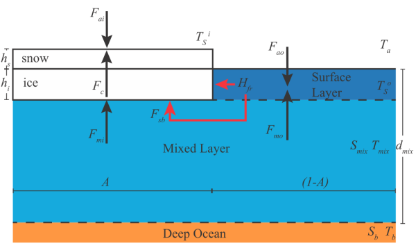1.

We used the Semtner (1976) zero-layer sea ice model, which assumes a linear temperature gradient through the snow and sea ice. i.e. no internal storage of heat by the sea ice (NOT true in reality!). 2. The mixed layer component is based on the bulk mixed layer model of Kraus and Turner (1967) and Niiler and Kraus (1977), which assumes that temperature and salinity are uniform throughout the mixed layer (i.e. it is perfectly mixed), and there is a full balance in the sources and sinks of turbulent kinetic energy (TKE) within the mixed layer (no loss of energy). 3. This is coupled to a simple deep ocean, where the temperature and salinity of the ocean varies with depth.

An idealised model is useful in such an analysis for a number of reasons: 1. Its simplicity means we can completely understand the results of the model. 2. Its computational efficiency (runs very quickly!) allows us to perform a large number of sensitivity studies, whereby we vary different parameters (i.e. snow thickness) to understand how each in turn impacts the mixed layer evolution. 3. It works!

Through several case studies, the model simply demonstrated that atmospheric forcing differences were SUFFICIENT to explain the bimodal distribution. The simplicity of the model means other mechanisms (e.g. regionally varying ocean dynamics) still cannot be neglected.

See my paper about this idealised model here.

CICE Modelling

To more realistically represent the Antarctic sea ice, and to extend the work to the entire Southern Ocean domain, we also used CICE, a sea ice climate model component developed in Los Alamos.

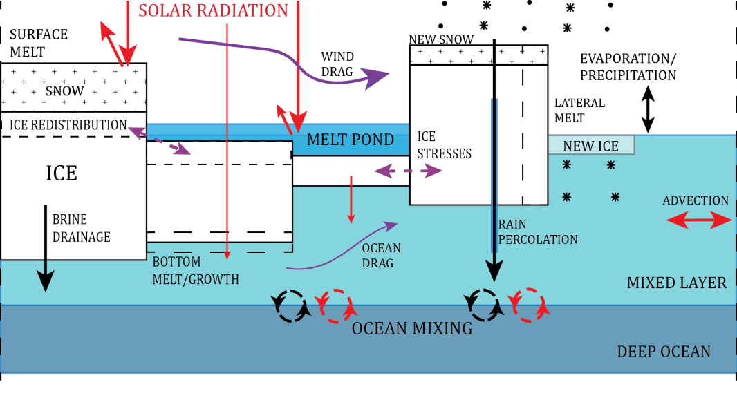
I coupled CICE to a simple mixed layer model (similar to the one used in the idealised study above) to look at the mixed layer evolution of the entire Southern Ocean. A schematic of the sea ice thermodynamics used by CICE (and the mixed layer model we coupled to CICE) is shown on the right. We can see that the simple sea ice model has been replaced with a multiple thickness category sea ice scheme, including a number of advanced thermodynamic parameterisations that play important roles in the growth and melt of sea ice (basal/lateral melt, ridging, snow-ice conversion etc).

Using this model, we highlighted regional differences in the behaviour of the sea ice and its impact on the ocean surrounding Antarctica. Specifically sea ice was shown to play the crucial role in the seasonal evolution of the surface mixed layer (through the brine fluxes as sea ice grows and melts).

See my paper about this CICE model study here.

Extra Background Material

The Mixed Layer

An important feature of the oceans is the top surface layer of constant(ish!) salinity, temperature and density, known as the mixed layer. The figure below demonstrates the variety of processes taking place on top, below and within the mixed layer.

The mixed layer maintains its constant profile through turbulent mixing at the ocean surface, as a result of wind stirring and buoyancy fluxes. As it is the part of the ocean affected most directly by changes in atmospheric conditions, the mixed layer can show strong seasonal variability. Through a release of dense salty water (when sea ice forms in winter), we can see the mixed layer deepen in the winter (negative buoyancy flux), and through the addition of freshwater in the summer (melting of the sea ice) we expect the mixed layer to shallow (positive buoyancy flux).

A higher wind velocity will increase the ocean surface stress which, as well as driving more turbulent mixing at the surface, can also provide a constant source of open water generation as the ice is being constantly exported. This process is strongest in coastal polynyas, where a permanent open water region is maintained through the rapid export of sea ice. Winds therefore play an important direct and indirect role in the mixed layer evolution.

Sea Ice

Sea ice covers a large fraction of the Earth’s surface. It is found in both the northern and southern hemispheres and its extent shows strong seasonal (and potentially annual) variability. Sea ice formation is a complex process and is in itself still an active area of research. The turbulence of the ocean and the salinity of the sea water means sea ice forms very differently to that of pure ice.

The salinity of sea water lowers the freezing point of the water. For the salinities we find at the ocean surface (~34 parts per thousand) we expect a freezing temperature of around -1.8C (pure water freezes at 0 degrees C of course!). Sea ice retains some of this salt in brine pockets which significantly impact its thermal properties. Some of this brine is drained away (mainly through either gravity drainage or surface meltwater flushing). Sea ice therefore always maintains some kind of bulk salinity (a rough approximation of 5 parts per thousand is often used in global climate models).

The sea ice acts as an insulating lid over the ocean, controlling the transfer of heat, salt and momentum to the atmosphere. Understanding sea ice is therefore crucial if we want to understand the evolution of the Antarctic shelf seas which are covered by sea ice virtually all year round.

Ice Shelves & Sea Level Rise

Scientists have recently observed a rapid ocean-driven thinning and acceleration of the Pine Island Glacier in the Amundsen Sea embayment, West Antarctica. The acceleration of this glacier into the ocean means that the glacier is losing grounded ice to the ocean faster than it is being replaced by new ice (itself formed through snow compaction), raising sea levels by a few millimetres each decade. A collapse of the ice shelfm however, could open up the ice sheet to rapid ice loss through these fast moving streams of ice, where a complete disintegration of the West Antarctic Ice Sheet has the potential to raise global sea levels by around 3m (the East Antarctic Ice Sheet has the potential to raise sea levels by upwards of 50m!).

It is believed the rapid thinning of the Pine Island Glacier is driven mainly by warm ocean currents below the ice shelf. These warm ocean currents are only found in specific regions surrounding Antarctica, meaning ice shelves in other regions (such as the much larger Filchner-Ronne Ice Shelf in the Weddell Sea) are better protected from the warm ocean waters circumnavigating Antarctica. Recent modelling studies however have suggested that in a warming climate, a thinner sea ice cover in the Weddell Sea could allow for warm waters to flood onto the Weddell continental shelf in the future, providing another possible route for rapid ice loss and sea level rise from Antarctica.

There is still great uncertainty surrounding the future stability of the Antarctic ice sheet, meaning new observations and improved modelling of this region is urgently required.